Here is a different style of map that I don’t use very often. It is a 3D view of the Maracas Watershed, Trinidad.
The purpose of this map is just to appreciate the topography of the watershed. Its interesting that the headwaters of the valley is pretty wide, then narrows moving downstream towards the Caroni River.
This was my first time trying to create anything 3D. I used the DEM as the elevation source, and made it slightly transparent to view the Open Street Map basemap underneath. I thought of applying contours but it just looked too messy.
I usually don’t like “3D” as a lot of detail is lost when viewing on a 2D medium, but here we can appreciate the heights of the surrounding hills, with the second highest peak in Trinidad, El Tucuche, in the background. This map would be much more interesting as a 3D model.
In honour of Carnival and Panorama season, here is a map of the Large Steelbands in Port-of-Spain. Special shout out to my old band – Silver Stars. I definitely miss the excitement of Carnival.
Now there’s some info in there that’s not correct and some that’s just vague. Luckily I know where most of them are and Google knew the rest. I had no idea Desperadoes now have a fancy permanent yard.
The challenge here was deciding what to put on the map. Putting all bands on the map would require a small scale and only give the general location of the band. By zooming in on the Northern region, the user can see the precise location which I think is more useful.
This one shows all of the Large and Medium bands in Trinidad and Tobago. Did not attempt to do the Small or Single Pan bands as I (or Google) don’t know most of them but that would be nice addition someday.
The Adopt-A-River maps are clean and easy to read. I added a basemap to provide more context and also wanted to decrease the size of the legend. Used the Open Street Map basemap as the others seemed to think the Caroni Swamp didn’t exist.
I wanted to keep the watershed labels constrained to inside of the features, but as you can see Lower Navet is trying to escape. I also added rivers but did not label them as I think that would be too cluttered. The large empty space on the left was also interesting to try to fill.
A few years I put together an interactive watershed map here:
In the Viewing the Results post, we saw the neat Particle Tracing feature in RAS Mapper, which us to easily visualize the movement of water. However, if we look closely enough, things look a bit strange. The particles seem to be going straight through that road embankment (The Priority bus Route) as if it doesn’t exist.
Original Particle Tracing
Now we know that the Priority Bus Route does in face exist but the model does not know that because the current cell faces do not align with the embankment. The model only sees what the cell faces see, and so since the faces do not fall on top of the road embankment, it pretty much does not exist in the model. This means our model is not very accurate, which we already know.
To get the cell faces to align with the the road embankment, Breaklines are used. Breaklines force the mesh to follow the user-defined line, and can be added at any time during the mesh development process. Breaklines should be added to any location that is a barrier to flow, or controls flow/direction such as levees, roads, and natural berms in the terrain. In the screenshot below, I have added (and enforced) two breaklines over the two main road embankments. Now the particle tracing and floodplain shape look very different.
Particle Tracing with Breaklines added
First we notice that there is faster velocity through the structure opening as expected as water speeds up to squeeze through. We also see that water does not seem to be just passing through the embankment like before (expect on the left side which suggests the road is overtopping). Lastly, we notice that the floodplain upstream of the road is much larger than previous, while the downstream is smaller as water builds up behind the road.
It is obvious that Breaklines make a big impact on model and definitely help to improve its accuracy. The next questions is: where do breaklines come from and how to process them to import them into RAS. To be continued…
From the previous post, we saw that water was not leaving the model, causing a build up of water at the downstream end (although the downstream end is the Caroni Swamp where we expect water to be). To fix this, we add a Boundary Condition Line at the downstream end of the model.
in RAS Mapper, start editing the Geometry. Turn on Boundary Condition Lines and select it to draw a new feature. I turned on the max Depth results grid to use as a guide. Draw the Boundary Condition Line left to right, looking downstream. Ensure that the maximum extent of the floodplain is covered so that it can properly drain. I have named the line Outlet.
Boundary Condition Line at the basin outlet
Now we need to set the type of Boundary Condition to apply to the newly drawn line. Save edits and close RAS Mapper. In the Unsteady Flow File, the line will be added to list of boundary conditions. We will set the boundary condition to Normal Depth, which allows the water to flow freely from the model.
Normal Depth assigned to Outlet
Double clicking on Normal Depth allows us to set the value to 0.0001. This represents a very flat slope, which represents the flat topography of the swamp where water is not expected to move very quickly.
Normal Depth set to 0.0001
the Normal Depth Boundary Condition Line is ready to go! Run the model again. Interestingly, the model runs slightly faster than previous, possibly because there are less wet cells as water can now exit the model.
Runtime Message with the Normal Depth Boundary Condition
Now to compare results. below the previous results are on the left and the results with the Normal Depth applied are on the right. The Normal Depth shows less water in the model as we can see that the Highway is no longer submerged and the general floodplain extent is smaller.
Normal Depth Comparison at End of Simulation
We have successfully added a Normal Depth Boundary Condition at the downstream extent of our model. In the next step, we will be adding more detail to the 2D mesh using Breaklines. In the previous post there was a screenshot of the particle tracing showing water going through a road (as opposed to over or around it as one would expect). It would be great it that didn’t happen.
Now for the fun part! Now that we have successfully run the RAS model we can take a look at the results. This is easily done in RAS Mapper, which has several different options for viewing the spatial results.
Under the Results section, the ShortID of the event if shown along with Depth, Velocity, and Water Surface Elevation grids. These are set to the Max profile by default. This may not correspond to a single time step, but shows the maximum values at any cells over the entire simulation.
Max Depth
Use the time slider at the top of the window to pan through the simulation to see how the results change. An animation of the simulation can also be played.
Depth at the End of the Simulation
Particle Tracing is another fun way to visualize the results. This cannot be done on a Max profile as these results may be compiled from several different time steps, so a single time step must be chosen using the time slider. Particle tracing helps to visualize the movement of water over the terrain.
Velocity Particle Tracing
There are several other results that can be added to RAS Mapper. Right-click on the event and select Create a New Results Map Layer. Options such as the Froude Number, Shear Stress, Arrival Time, and many others can be added to the map. We will go over a few of these in later posts.
Looking at the Depth results at the end of the simulation, we notice that there is a build up of water in the Caroni Swamp (The Caroni-Arena dam is also clearly visible). Now we know that there is water perpetually in the swamp, but nevertheless we want our model to freely drain for now. In the future we can consider the tidal conditions, but for now if we want water to leave our model, we need to add Boundary Condition Lines.
The Plan file contains the settings used to run the model such as the simulation window, what time steps to use, and what equation sets to use. The main things that we will do for now is ensure that the geometry and Unsteady Flow files are associated, and enter the Simulation Time Window.
Here I have named the Plan file 100yr as that is the event we will be running. The Short ID is used to display the Results and is also used as the Part F in the output DSS file.
The Simulation Time Window should cover the Time of Concentration of the watershed. There are equations out there to calculate the time of concentration, but for now I will just guess that it is less than 2 days. Starting it on 01Jan2000 is arbitrary as this is a hypothetical event. If we were simulating an actual historical event, the Simulation Time window would match the event.
There are other options we can tinker with that can improve model stability but we will cover those later. For now we just want to run the model.
Unsteady Flow Analysis
Once you have entered the simulation window for the event, press Compute to run the model!
Runtime Messages
A new window will popup with the Runtime Messages. Here it gives a brief summary of the settings used in the model and gives the status of where it is in the model simulation. This model took 13 minutes to run on my computer, which is pretty quick for a 2D model, which can run for several hours. We also see the Volume Accounting Error is low which is good. If it were over 2% we would start to get worried that water is being lost in model that is not accounted for.
Now that we have successfully run the model we can View the Results.
Now we will set the rainfall that will be applied to the mesh during the simulation. I will most likely have a few posts on how to actually go about developing this rainfall table, but the goal for now is just to get a working model and then make it better. So in interest of time I will skip over the scientific hoopla for now and just make up some numbers.
We need to create and Unsteady Flow File before adding precipitation. The Unsteady Flow File contains the inputs and output conditions of the model. The unsteady part means that these conditions are changing over time, as opposed to a Steady Flow File where the conditions are constant. I have named this file 100yr as I intend to derive the 100yr rainfall from somewhere eventually.
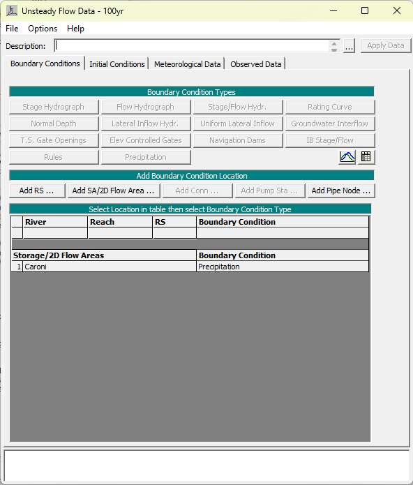
Unsteady Flow Data Editor
Click on Add SA/2D Flow Area and add the mesh we created. Precipitation is the only boundary condition available to apply to 2D Flow Areas and luckily that is what we want. Clicking on the Precipitation boundary condition brings up the Hyetograph Editor.
Precipitation Hyetograph Editor
As you can see, I have set the Data time interval to 1 hour since that’s a nice round number. Typically for floodplain mapping applications, we use the 24 hour storm, which means a storm that lasts for 24 hours. For most storms, we expect the bulk of the rainfall to occur in the middle of it so that is what is have done here. The total rainfall depth is 191mm, which is a modest hurricane. Again I intend to do a full statistical analysis of actual rainfall data. This are just made-up, although educatedly guessed, numbers.
Precipitation Hyetograph
Clicking on Plot Data allows us to view the Hyetograph, and we can see that it has a typical shape, although a bit clunky at the bottom. The peak hourly rainfall is 100mm, which is certainly enough to flood Port-of-Spain.
Our Precipitation is ready to go! The next step is to define the simulation settings and run the model.
The mesh is what makes it a 2D model. Read the RAS documentation to learn more about the properties of the 2D mesh including computation points and cell faces. In a 1D model, rivers are modelled using cross-sections across the floodplain, distributed along the river. In a 2D mesh, I think to think of the cell faces as 1D cross-sections, and the cell center as a storage area that receives precipitation and allows for infiltration.
I have chosen to do a 2D model here because the lower portion of the Caroni watershed is a very wide and flat floodplain, and I expect there to be multiple flow paths. Also because I prefer doing 2D models. Now if we were modelling just the Maracas Valley or the Aripo Valley, a 1D model can give just as good results as a 2D model since flooding is contained to the channel. I intend to test this at some later date, but for now we carry on with the 2D model of the Caroni basin. Check out Chapter 6 in this document on the advantages of 2D modelling over 1D.
Import the Basin Boundary
which we delineated as one of the first steps of this project. In RAS Mapper, start editing our geometry, right click on Perimeters > Import Features From Shapefile. A wizard will pop up and you can select the boundary shapefile to be imported. If no features show up you may have incompatible features, usually meaning multipart features.
Importing the Basin Boundary from shapefile
Generate Computation Points
Once we have successfully imported the perimeter, we can generate the Computation Points. We need at least one perimeter to generate the points. A model can have more than one perimeter for more complex models, but here we will just stick with one.
Right click again on Perimeters > Edit 2D Area Properties. Here we need to set the general spacing of the points, which is the distance between them. The rule of thumb is to select a size that can accurately capture the topography of the terrain without sacrificing model runtime. A model with a million points will run much slower than one with a thousand points. Here I chose 100 meters since its one of the more popular Olympic track and field events. Later we will add more detail to the mesh.
2D Flow Area Editor
Face Perimeter Connection Errors
After generating the points, you may notice that the mesh has Face Perimeter Connection Errors. These occur at sharp bends in the perimeter where the general point spacing cannot account for the angle in the perimeter. These are identified by large red dots on the problem points. These can be solved by adding Computation points in the area, or adjusting the perimeter to be smoother. In the screenshot below I added on point and the problem went away.
Face Perimeter Connection Error
Save the Geometry once all the errors have been resolved, indicated by no error messages at the bottom left of the window The 2D Area properties will also not mention any errors.
Our 2D mesh is ready to go! It has 87006 cells in it. Of course, there are several things that can be done to add more detail to the model such as adding breaklines and refinement regions, but for now we just want an error-free mesh to run the model. The next step is to apply some rainfall to it.
Now that we have a project setup and a projection defined, we can import the terrain. It is recommended that you clip the terrain raster to a buffer of the basin boundary. I used a buffer of 1km because if any part of 2D mesh extends beyond the terrain, the model will not run. I used Extract by Mask in ArcPro to clip the terrain raster.
In RAS Mapper, right click on Terrain and select Create a new RAS Terrain. Point to the clipped terrain and hit Create. RAS may take some time to import the terrain, depending on its size and resolution.
Once the terrain has been successfully imported, you can explore it in RAS Mapper. Turning on the Update Legend with View property makes it easier to see the changes in elevation.
Maracas Valley
Add a New Geometry
Next, we will create the geometry file that will be used to develop the 2D mesh. Right click on Geometries and select Create New Geometry. Give it a descriptive name. I have named this Geometry 2018ExistingConditions since that is when the LiDAR was developed. Under Geometries, you can see all the available components that can be used to develop the model geometry. We will go over these eventually. For now, save the empty geometry.
Manage Geometry Associations
We need to tell RAS to apply the Terrain to the geometry that we created. This is important when we have multiple geometries or multiple terrains that we are testing. Right click on Geometries and select Manage Geometry Associations. Ensure that the Terrain is matched with the geometry. You can see that there are other layers that are currently missing. They are not required to run a 2D model but may help to make the model more accurate
Manage Geometry Associations
Now that we have a terrain, the next step is to create the 2D mesh.
The Beetham Landfill is surprisingly much high than its surroundings