Now we will set the rainfall that will be applied to the mesh during the simulation. I will most likely have a few posts on how to actually go about developing this rainfall table, but the goal for now is just to get a working model and then make it better. So in interest of time I will skip over the scientific hoopla for now and just make up some numbers.
We need to create and Unsteady Flow File before adding precipitation. The Unsteady Flow File contains the inputs and output conditions of the model. The unsteady part means that these conditions are changing over time, as opposed to a Steady Flow File where the conditions are constant. I have named this file 100yr as I intend to derive the 100yr rainfall from somewhere eventually.
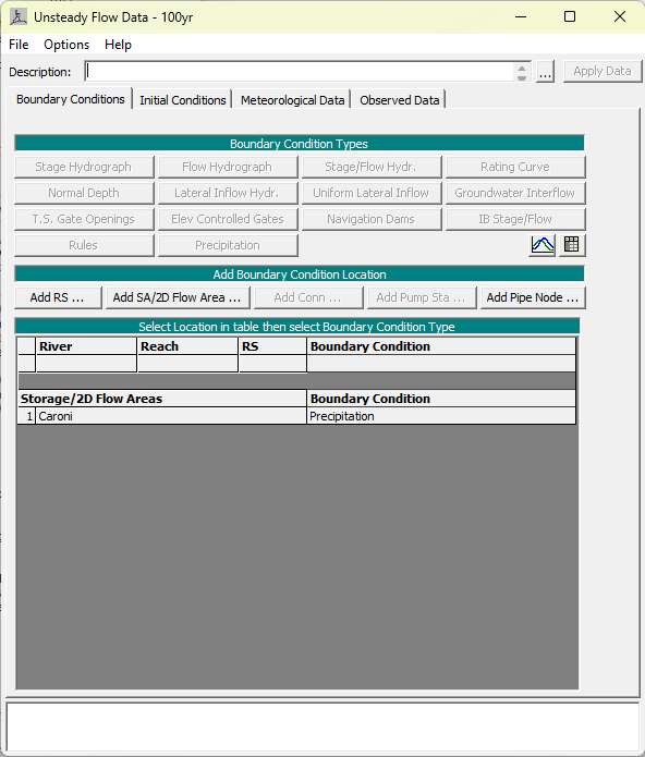
Click on Add SA/2D Flow Area and add the mesh we created. Precipitation is the only boundary condition available to apply to 2D Flow Areas and luckily that is what we want. Clicking on the Precipitation boundary condition brings up the Hyetograph Editor.

As you can see, I have set the Data time interval to 1 hour since that’s a nice round number. Typically for floodplain mapping applications, we use the 24 hour storm, which means a storm that lasts for 24 hours. For most storms, we expect the bulk of the rainfall to occur in the middle of it so that is what is have done here. The total rainfall depth is 191mm, which is a modest hurricane. Again I intend to do a full statistical analysis of actual rainfall data. This are just made-up, although educatedly guessed, numbers.

Clicking on Plot Data allows us to view the Hyetograph, and we can see that it has a typical shape, although a bit clunky at the bottom. The peak hourly rainfall is 100mm, which is certainly enough to flood Port-of-Spain.
Our Precipitation is ready to go! The next step is to define the simulation settings and run the model.
